

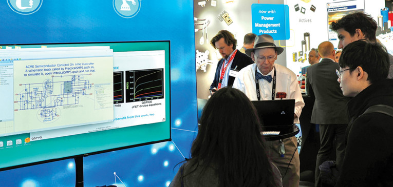
In 2020, Mike (now associated with Marcus Aurelius Software, LLC) created QSPICE (the Q is for Qorvo, the company that supported the new effort), which he defines as the simulation tool suite he would have written 25 years ago if he knew then what he knows now, and if he had access to the hardware and software technology that is available today.
Offering a faster and easier to understand user interface, the QSPICE circuit simulator is being praised for the ability to handle complex analog and digital designs seamlessly while contributing to energy-efficient circuit development. Mike predicts that QSPICE will become the most popular simulation tool, surpassing all others combined.
While earning his undergraduate degree at the University of Michigan and graduate degree at the University of California, Berkeley, Mike Engelhardt’s early work involved designing electronics for physics experiments, and creating sophisticated, custom-built equipment. “The electronics in physics experiments is not off-the-shelf equipment,” he says. “You have to design and make a lot of fairly fancy stuff, and that’s how I learned electronics. I was also very interested in simulation from a very early age because I just thought it was really fascinating as a way of solving technical problems that couldn’t be solved by any other means.”
Mike says the role of simulation in engineering is often misunderstood. He emphasizes that simulation should be used to gain insight into circuit behavior rather than just verifying designs. “The point of simulation is to nurture your intuition, to develop your understanding of a circuit,” he explains.
Mike Engelhardt is well aware of the popularity of LTspice among audio designers, and he is very keen to share the details about how QSPICE helps address audio challenges even better. On the DIYaudio forum, he interacts frequently with members to support projects and promote education. Recently, I had the opportunity to ask him a few questions.
Tim McCune: There’s a great interest in measuring distortion in audio circuits. What would be the best way to measure it, is that a Fast Fourier Transform (FFT)?
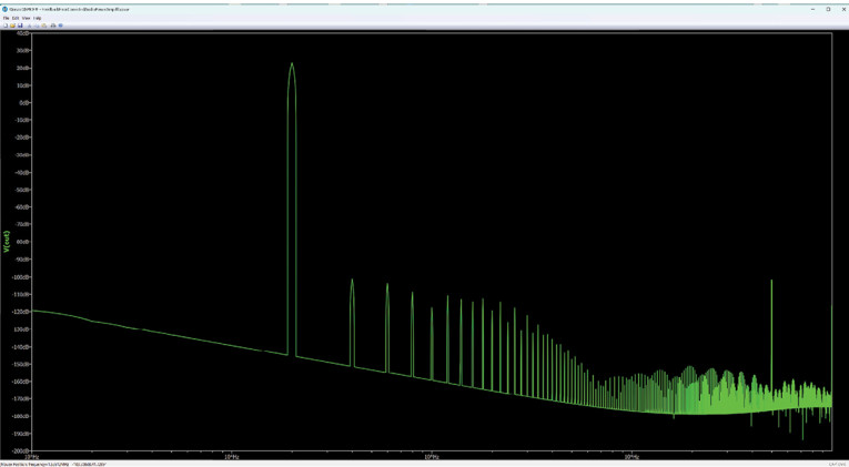
Mike Engelhardt: The thing you need to know about distortion measurement in QSPICE is that there’s actually an older method before FFT, called .four, that was popularized by PSpice. With the .four directive QSPICE would look at the last period of your simulation; for instance, you might simulate 10ms with a 1kHz test signal. And it would look at the end of the data and then go back exactly 1ms and compute the Fourier components of 1kHz, 2kHz, 3kHz, etc., up until the default at 9kHz, and then sum those nine harmonics and compare it to the fundamental and give you a total harmonic distortion figure. Figure 1 shows a representative example.

The .four method predated FFT in SPICE because I think when people developed the .four directive they were not familiar with the FFT, because it is a fairly sophisticated algorithm, even though the FFT method predates SPICE by about three years. As far as I know, FFT is from about 1965 and SPICE was developed around 1968, so FFT was definitely high-tech math, and it wouldn’t have bled over to the electrical engineering department yet at the time.
The FFT reveals the frequency content of a time domain simulation — much like a spectrum analyzer. But unlike a spectrum analyzer, the FFT data is complex, meaning it includes phase information though that usually isn’t useful. When you do an FFT in QSPICE, the phase information is turned off by default, but you can turn it on. For example, if you do an FFT of a tank circuit ringing down, the phase plot of the FFT isn’t meaningless. That result is used in some instrumentation, such as that used down-hole in oil exploration. Figure 2 is a representative example of an FFT result.
ME: I generally like the FFT; what’s nice about the FFT is that usually I can just look at one or two harmonics that are of interest and compare them to the magnitude of the fundamental. That’s very straightforward, but if you want to know the total harmonic distortion that you put in a specification, then use the .four directive because that will most likely be the least error-prone method.
TM: With QSPICE are we looking at anything new with respect to FFT and how users see this in the simulation?
ME: The most important improvement is that QSPICE doesn’t compress the waveform data, and it knows what time steps to take. So, if you’re going to measure total harmonic distortion at 1kHz as is typical or more critically at 20kHz, QSPICE will take a time step such that the noise floor will be down by your RelTol parameter.
If you set RelTol to say 0.001, and if you just do a simulation, you have 60dB (a factor of 1000) of dynamic range in making your total harmonic distortion measurement. If you set RelTol to 10 to the minus 4, your noise floor is down to 80dB. There’s a simple, transparent, and straightforward relation between the tolerance you ask for and the noise floor from your Fourier analysis. And that improved accuracy goes for both .four and FFT.
TM: You’ve talked a bit about compression of the waveform. Can you delve in a bit further?
ME: A SPICE simulator generates a huge amount of data, more data than typical computer hardware can plot, even using single pixel wide lines. If you just use single pixel wide, you can plot that pretty fast, but that doesn’t look good on a computer screen. So, you usually use lines that are more than a single pixel wide, and at that point a CPU takes a very long time to plot that. That’s what most SPICE programs use; they do most of their graphics with the graphics processing unit (GPU) of the PC.
Use of the GPU is an integral part of the design of QSPICE. The point is that even a modest GPU can plot lines 100,000 times faster than a CPU. This means there’s no reason to compress the waveform data and the FFT noise floor stays at the intrinsic limit of the simulation.
But even though you have that GPU, most SPICE programs don’t use it, they actually use an older graphics library that renders everything with the CPU and then draws that to the graphics memory. That’s very slow. If you have even a mediocre graphics card, it can plot lines beautifully, dithered like desktop publishing quality lines. QSPICE doesn’t even bother using compression because, instead of trying to speed things up by a factor of 10, it goes straight to the jugular with the GPU and gets a factor of 100,000 speed over CPU graphics.
ME: Yeah, I’m leveraging gaming hardware. The GPU business is driven by teenagers’ video gaming needs. So, you have these gaming PCs, and I’m just using that hardware for QSPICE. The simulator I have written uses gaming hardware very efficiently.
But even if you don’t have gaming hardware, it still uses the GPU that every PC has. Even if you have a low-performance graphics processor in your notebook, you’re still going to see a huge improvement over trying to render your stuff with a CPU.
TM: What’s your approach in calculating and presenting harmonic distortion information in QSPICE?
ME: For calculation of the THD of an audio amp, I still kind of like the old-fashioned .four statement, which I think is due to PSpice. It doesn’t use an FFT but just looks at the fundamental and specific harmonics. Then it reports the THD (Figure 1). For anything besides THD, I like the view that an FFT yields (Figure 2).
When using the FFT method, you can look at how far a specific harmonic is below the fundamental. So, you drag a box in the waveform viewer of the FFT data from the peak of the fundamental down to the peak of some harmonic. You look at the status bar, and it will tell you the difference as a ratio.
If you’re in QSPICE, if you’re looking at the differences in complex data, it isn’t actually differences but ratios, because complex data is from a linear system, so the actual absolute difference doesn’t matter. It’ll be the relative difference in decibels, which is the ratio of magnitudes. And that’s how you do it if you’re doing the FFT method.

ME: The nice thing about QSPICE for THD work is that it knows how to compute step size for a sine wave test signal, as I previously mentioned. If you’re going to do a test of a continuous-time audio amplifier, some Class A or Class AB amplifier with no switching in it, then you should not have to adjust the step size. You should be able to simply ask for a tolerance through RelTol, which will default to 60 dB, and you can do your simulation. If the test signal is a sine wave source, like a voltage source or a current source — then QSPICE knows what time-step size to take, such that every data point between step sizes is within the test waveform.
Not only the individual points are correct, but every point between two time steps can be approximated with a straight line and be within the tolerance you ask for. And that should all work. And if the result seems off, go to a small step size by decreasing RelTol and see if you get a different number.
TM: How does this approach help users understand circuits and design decisions better?
ME: It’s simple and less error-prone, right? There’s no compression to defeat, and setting the tolerance is straightforward and transparent. In other SPICE simulators, you must stipulate some absurdly tiny step size which isn’t related in a straightforward way to the FFT noise floor.
TM: When you started talking about improved models/device equations for QSPICE, you mentioned including sub-threshold conduction measurements for JFETs and MOSFETs. Bob Cordell told me this is an important improvement, that having a model where transconductance suddenly goes to zero doesn’t work well for these parts.
ME: Well, for me, subthreshold conduction does three things for you — and what Bob Cordell is talking about is absolutely true. First, it makes finding the initial DC operating point easier. Without sub-threshold conduction, the differential behavior of the FET disappears once Vgs is below the threshold voltage and the simulator no longer knows how to iterate to the solution.
The second thing it does is eliminate the non-physical abrupt turn on/turn off of a FET inside of a time step. That nonlinearity makes integrating the differential equations with a second-order method flaky and can initialize a trap ringing episode. And of course, the third thing is that FETs have subthreshold conduction, often so much you can see it in a curve of the output characteristics, so the simulation is more correct.
Sub-threshold conduction makes solving the circuit easier because when SPICE solves your circuit, it looks at the differential behavior on all the devices from different voltages. And so, knowing how a voltage change — how one voltage changes another voltage — is the way it solves the circuit.
But if you pinch off a FET so that the gate-source voltage is below the threshold voltage, it doesn’t matter what the gate voltage is. There’s no change in behavior of the circuit. So, SPICE simply cannot solve for the circuit in that condition. It has no idea what the gate voltage should be.
Now, another thing it does for you is — and this starts addressing Bob Cordell’s concern — that it eliminates the abrupt turn on and turn off of a FET. If you don’t have subthreshold conduction, you’ve added an artifact of the behavior of the FET that it snaps on and snaps off. And if that happens during a time step, you can’t integrate the differential equations that arise from the reactance of the circuit with a second-order method with that discontinuity. And you don’t know that discontinuity happens.
TM: That’s a change in the modeling of FETs that’s in QSPICE, right?
ME: QSPICE supports subthreshold conductions for both MOSFETs and JFETs. Okay. So, you know, that’s actually new. I don’ t know of another simulator that’s ever been written that includes subthreshold conduction on a JFET. To the best of my knowledge, that’s not been done before. aX
This article was originally published in audioXpress, March 2025